Kevin Hua

Principal Component Analysis

Introduction

Before transferring, I took an introductory course to linear algebra in Spring 2021 at the University of Buffalo. I enjoyed that class very much, although the class was delivered online due to the pandemic. After I transferred, with great interest in linear algebra, I took a more advanced proof-based linear algebra class in Winter 2022 that underscored linear transformation and its geometric interpretation. It was wonderful. After the class ended, I decided to learn more on my own.

Principal Component Analysis (PCA) is one of the most important applications of linear algebra in Machine Learning. However, there is so much involved that it might appear discombobulating to those new to this subject.

I, therefore, collect all my study notes regarding this subject and compile them into this document as a tutorial, which I hope you will find helpful!

Note: there are various fashions to do principal component analysis. But, here, we will limit the scope and only zero in on one method – through deriving sample covariance matrix and change of variables.

Observation vectors and the matrix of observations

An observation vector is a vector that records the measurements of properties that we are interested in on our objects. More specifically, each entry of the vector specifies a measurement of one of the corresponding properties. For example, if we sample a group of students. And we measure each student’s weight and height. One observation vector, \(\textbf{X}\), will be created for each student to contain their weight and height, denoted as w and h, where \[\textbf{X} = \begin{bmatrix} w \\ h \end{bmatrix} \] As its name suggests, a matrix of observations consists of a collection of observation vectors (we assume there are n students). It has the form \begin{bmatrix} \textbf{X}_1&\cdot\cdot\cdot&\textbf{X}_n \end{bmatrix} where \[\textbf{X}_i = \begin{bmatrix} w_i\\ h_i \end{bmatrix} \]

Sample Mean and Mean-deviation form

Before we delve into PCA, we have to talk about deriving the sample covariance matrix. But before that, to derive the sample covariance matrix, we need to derive the \(\textbf{sample mean, M,}\) of the observation vectors \(\textbf{X}_1,...,\textbf{X}_n\) is defined as \[\textbf{M = } \frac{1}{n}(\textbf{X}_1 + \cdot\cdot\cdot + \textbf{X}_n)\] Before proceeding to compute the covariance matrix, the original observation matrix has to be transformed into mean-deviation form \({B}\), where \[B = \begin{bmatrix} \hat{\textbf{X}}_1&\hat{\textbf{X}}_2&\cdot\cdot\cdot&\hat{\textbf{X}}_n \end{bmatrix}\] where \[\hat{\textbf{X}}_k = \textbf{X}_k - \textbf{M}\] for each 1 \(\leq\) k \(\leq\) n.

It’s known that \({B}\) has a zero sample mean. But why is it zero? Below is the proof.

Let the sample mean of the columns of \({B}\) be \[\hat{\textbf{M}} = \frac{1}{n}(\hat{\textbf{X}}_1 + \cdot\cdot\cdot + \hat{\textbf{X}}_n)\]\[ = \frac{1}{n}(\textbf{X}_1 - \textbf{M} + \cdot\cdot\cdot + \textbf{X}_n - \textbf{M})\]\[ = \frac{1}{n}(\textbf{X}_1 + \cdot\cdot\cdot + \textbf{X}_n - n\textbf{M}) \]\[ \hspace{9cm} = \frac{1}{n}(n\textbf{M} - n\textbf{M}) = 0 \hspace{8cm}\square\]

A positive semidefinite covariance matrix

Now, we can substitute \({B}\) into the formula below to obtain our sample covariance matrix. \[S = \frac{1}{n - 1}{B}{B}^T \] Moving on, one might ask, “why is a matrix of the form \({B}{B}^T\) always positive semidefinite?” Below is the proof.
\[\vec{x}^T{B}{B}^T\vec{x} = \vec{x}\cdot({B}{B}^T\vec{x}) = ({B}{B}^T\vec{x})\cdot\vec{x} = ({B}{B}^T\vec{x})^T\vec{x}\] \[ = \vec{x}^T{B}{B}^T\vec{x}\] \[ = ({B}^T\vec{x})\cdot({B}^T\vec{x})\] \[ \hspace{10cm} = ({B}^T\vec{x})^2 \ge 0 \hspace{9cm} \square\] Hence, \({B}{B}^T\) is positive semidefinite. Then, how about \({B}^T{B}\) ? \[\vec{x}^T{B}^T{B}\vec{x} = ({B}\vec{x})\cdot({{B}\vec{x}})\] \[ \hspace{10cm} = ({B}\vec{x})^2 \ge 0 \hspace{9cm}\square\] It turns out that \({B}^T{B}\) is positive semidefinite as well! Note that if \({B}\) is n \(\times\) n and invertible, \({B}^T{B}\) is positive definite. Below is the proof.

As \({B}\) is invertible, \[ker({B}) = {\vec{0}}\] Thus \[{B}\vec{x} = \vec{0}\] if and only if \[\vec{x} = \vec{0}\] Thus, \[\forall \vec{x} \ne \vec{0}, {B}\vec{x} \ne \vec{0}\] In other words, \[\hspace{9cm} \forall \vec{x} \ne \vec{0}, ({B}\vec{x})^2 > 0 \hspace{9cm} \square\]
Thus, \({B}^T{B}\) is positive definite.

The elements of the matrix.

One might also cast doubts as to why the diagonal entries of the sample covariance matrix are the variances of corresponding variables while non-diagonal entries are the covariances of two variables. I wish the proof below would dispel your unbelief.
Assume a p \(\times\) n matrix \[B = \begin{bmatrix} \hat{\textbf{X}}_1&\hat{\textbf{X}}_2&\cdot\cdot\cdot&\hat{\textbf{X}}_n \end{bmatrix}\] in mean deviation form.

Let the sample covariance matrix be \[{S} = \frac{1}{n - 1} {B}{B}^T \] We denote the entry in \({i}\)th row and \({j}\)th column of \({S}\) as \({S}_{ij}\). Then, \[{S}_{ij} = \vec{e}_i^T{S}\vec{e}_j = \vec{e}_i^T(\frac{1}{n - 1}{B}{B}^T\vec{e}_j)\\ = \frac{1}{n - 1}\vec{e}_i^T{B}{B}^T\vec{e}_j = \frac{1}{n - 1}({B}^T\vec{e}_i)\cdot({B}^T\vec{e}_j)\] \[ = \frac{1}{n - 1}(\begin{bmatrix} -\hspace{1.7mm}{\hat{\textbf{X}}_1}^T- \\ -\hspace{1.7mm}{\hat{\textbf{X}}_2}^T- \\ \vdots \\ -\hspace{1.7mm}{\hat{\textbf{X}}_n}^T- \end{bmatrix} \vec{e}_i) \cdot (\begin{bmatrix} -\hspace{1.7mm}{\hat{\textbf{X}}_1}^T- \\ -\hspace{1.7mm}{\hat{\textbf{X}}_2}^T- \\ \vdots \\ -\hspace{1.7mm}{\hat{\textbf{X}}_n}^T- \end{bmatrix} \vec{e}_j)\] The \({i}\)th column of \({B}^T\) is a vector \(\vec{x}_i\) in mean deviation form, composed of all data values taken upon a sole variable \({x}_i\).

Thus, \[{S}_{ij} = \frac{1}{n - 1}(\vec{x}_i\cdot\vec{x}_j) \\ = \frac{1}{n - 1}(\begin{bmatrix} {x}_{i1} \\ \vdots \\ {x}_{in}\end{bmatrix} \cdot \begin{bmatrix} {x}_{j1} \\ \vdots \\ {x}_{jn}\end{bmatrix})\] \[\hspace{3cm} = \frac{1}{n - 1}\sum^{n}_{k = 1}{x}_{ik}{x}_{jk} = \frac{1}{n - 1}\sum^{n}_{k = 1}({y}_{ik} - \bar{y}_i)({y}_{jk} - \bar{y}_j) = \begin{cases} \mbox{Cov}_{y_i,y_j}, &\mbox{ if } i \neq j \\ \\ \mbox{Var}_{y_i}, &\mbox{ if } i \neq j \end{cases} \hspace{3cm}\square \] Please note that \({y}_{ik} - \bar{y}_i = {x}_{ik}\) where \({y}_{ik}\) is the \(\textbf{original}\) data value while \(\bar{y}_i\) is the \(\textbf{mean}\) of \({y}_i\).

Please also note that the proof above also incidentally explains why we have to convert the observation matrix into mean-deviation form -- we need it for substituting into the formula.

Now, we are ready to delve into the main point – principal component analysis (PCA).

My understanding of PCA

Essentially, the gist of PCA is eliminating redundant data by collecting sequence data points along new axes (new variables) with the biggest variance but no covariance. As, in fact, the bigger the variance, the more information it encapsulates (the bigger the variance, the wider the range of change this variable bears, and the more information it can carry). On the other hand, as covariances represent the correlation between variables, they could be considered repetitive information in this case. (Consider the case where two variables are closely related. We only need one of the two as with one, and we could predict the other with the one we have). Therefore, our goal is to assume the largest variance while eliminating all covariances (variables are uncorrelated to one another).

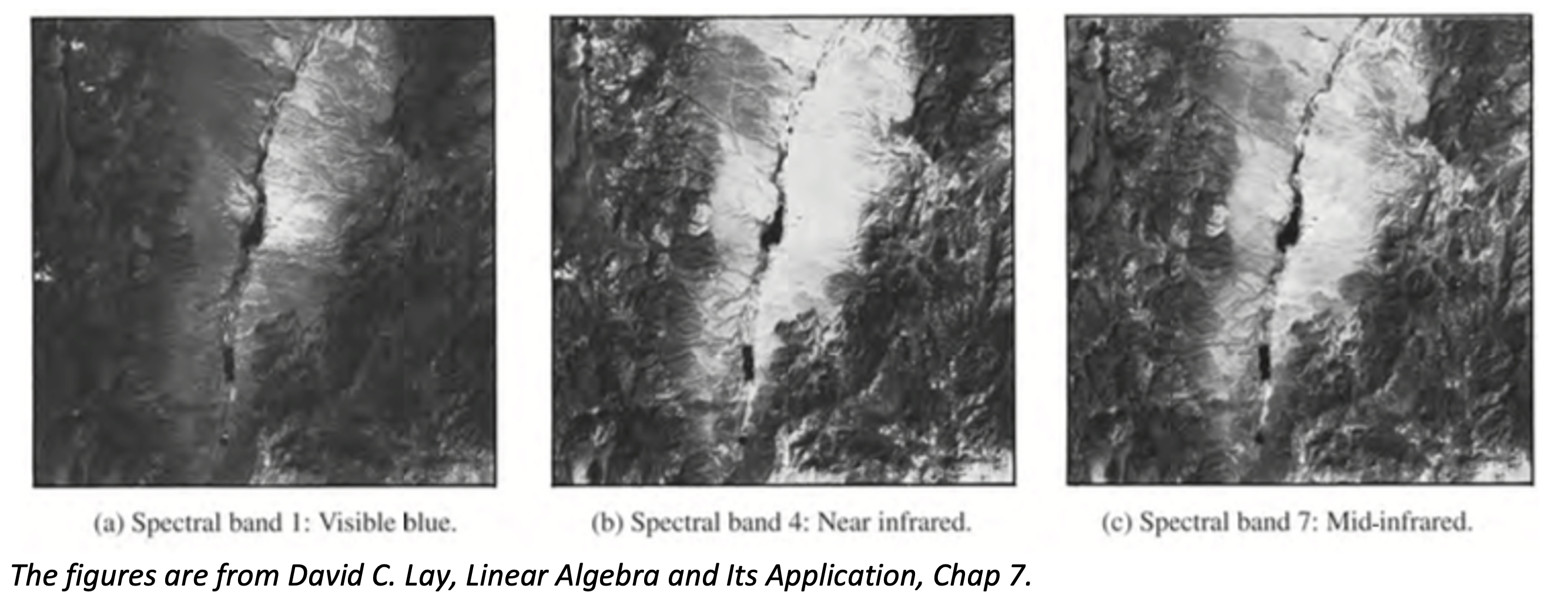
For example, let’s take a look at three shots of the same object, Railroad Valley, Nevada, where each of the three is captured with a different Landsat wavelength band.

As we can easily discern, some features of the valley appear in all three images, which are gratuitous. We can lessen the repetitions by boiling them down into a composite image with the aid of PCA.

At first, the three spectral components compose a series of observation vectors in \(\mathbb{R}^3\), where each entry of a vector records a pixel on one of the images.

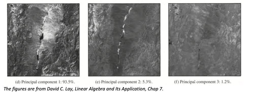
The goal of PCA now is to find three linear combinations of three spectral components. We can view those spectral components as different variables in the current coordinate system. And we want to do a change of variables to get to another coordinate system in which one of the new variables (linear combinations of the three spectral components) has the biggest variance. In this fashion, this new variable would embody most of the characteristics in all three images.

The original sample covariance matrix S represents the variances and covariances of data from (a) – (c).

Then, we would want a new covariance matrix (after the change of variable), maximizing the variances and minimizing covariances. As the sample covariance matrix is symmetric, it’s orthogonally diagonalizable. However, one might ask, why will this diagonal matrix do the trick? First, we are looking for a new coordinate system where variances are maximized, and covariances are minimized. With this in mind, it’s verifiable that this diagonal matrix would present the biggest variances in order, while it’s unquestionable that covariances are zero in this diagonal matrix. The justification can be found here.

In this fashion, the three-channel initial data can be reduced to one-channel data (d) (if we only want one channel, first principal component analysis), with a loss of a mere 6.5% of the scene variance. Basically, we only take the vectors along this sole axis.